Introduction
If you are anything like me, then you probably enjoy the contribution graphs that GitHub posts to both your own and others GitHub profile. You can see mine here. Since it is the beginning of a new year, I thought it would be fun to take a look back to see how I used GitHub in 2019 and in previous years. This is made much easier by using the gh R package which provides an R interface to the GitHub API. This post will walk through how to get all of the commits for your personal repos (so your results will look different from mine). The gh package will use the GITHUB_PAT environment variable to access any personal access token you have previously set up. If you do not have that configured, than you can provide your token with the .token argument.
library(tidyverse)
library(gh)
library(lubridate)
library(glue)
We will also define a custom color palette based on the GitHub Style Guide to stick with the post’s theme.
gh_pal <- c(blue = "#0366d6", yellow = "#ffd33d", red = "#d73a49", green = "#28a745", purple = "#6f42c1", light_green = "#dcffe4")Getting Repos
First, we want to get a listing of all of the repos that are associated with my GitHub account. We can do this using the /user/repos API endpoint.
repos <- gh("/user/repos", .limit = Inf)We can extract the desired information from the repos using the map_chr and map_lgl functions in the purrr package.
repo_info <- tibble(
  owner = map_chr(repos, c("owner", "login")),
  name = map_chr(repos, "name"),
  full_name = map_chr(repos, "full_name"),
  private = map_lgl(repos, "private")
)

# showing the first few non-private repos
filter(repo_info, !private)
## # A tibble: 35 x 4
## owner name full_name private
## <chr> <chr> <chr> <lgl>
## 1 saleslab DWC saleslab/DWC FALSE
## 2 saleslab ParsingLabSolutionsA… saleslab/ParsingLabSolutionsAS… FALSE
## 3 tbradley1… adv-r tbradley1013/adv-r FALSE
## 4 tbradley1… aob-power tbradley1013/aob-power FALSE
## 5 tbradley1… blog tbradley1013/blog FALSE
## 6 tbradley1… connectapi tbradley1013/connectapi FALSE
## 7 tbradley1… critical-thinking-ev… tbradley1013/critical-thinking… FALSE
## 8 tbradley1… dbp-calculator tbradley1013/dbp-calculator FALSE
## 9 tbradley1… dragondown tbradley1013/dragondown FALSE
## 10 tbradley1… dragondown_book tbradley1013/dragondown_book FALSE
## # … with 25 more rowsThere is a lot of other information contained within the repos API response. However, since I will be focusing mainly on my commits, I don’t need most of it for this purpose.
Get and Parse Commits
In order to get all of the commits for each of these repos, we will use the map_dfr to append all of the commit information for each repo into a single dataset. Before we do that, we need to define a few helper functions that can parse the output of the API endpoint response.
null_list <- function(x){
  map_chr(x, ~{ifelse(is.null(.x), NA, .x)})
}

parse_commit <- function(commits, repo){
  # browser()
  commit_by <- map(commits, c("commit", "author", "name"))
  username <- map(commits, c("committer", "login"))
  commit_time <- map(commits, c("commit", "author", "date"))
  message <- map(commits, c("commit", "message"))

  out <- tibble(
    repo = repo,
    commit_by = null_list(commit_by),
    username = null_list(username),
    commit_time = null_list(commit_time),
    message = null_list(message)
  )

  out <- mutate(out, commit_time = as.POSIXct(commit_time, format = "%Y-%m-%dT%H:%M:%SZ"))
  return(out)
}

gh_safe <- purrr::possibly(gh, otherwise = NULL)
The parse_commit function will extract the desired information from each API response. The null_list function is a simple helper to convert any NULL values in the response to NA, so that the map functions don’t throw errors. Finally, the gh_safe function is a safe version of the gh function. This is defined in case any of the individual responses fail, it doesn’t cause the entire loop to fail.
Now we can query all of the commits from each of these repos and filter the output to include only commits that I made.
all_commits <- map_dfr(repo_info$full_name, function(z){
  name_split <- str_split(z, "/")
  owner <- name_split[[1]][1]
  repo <- name_split[[1]][2]

  repo_commits <- gh_safe("/repos/:owner/:repo/commits", owner = owner,
                          repo = repo, author = "tbradley1013",
                          since = "2017-01-01T00:00:00Z",
                          until = "2020-01-01T00:00:00Z",
                          .limit = Inf)

  out <- parse_commit(repo_commits, repo = z)

  return(out)
})


my_commits <- all_commits %>%
  filter(commit_by == "Tyler Bradley") %>%
  mutate(commit_time = commit_time - hours(5))

my_commits
## # A tibble: 3,549 x 5
## repo commit_by username commit_time message
## <chr> <chr> <chr> <dttm> <chr>
## 1 nmanna/… Tyler Bra… tbradley… 2019-10-25 07:16:50 rendering changes
## 2 nmanna/… Tyler Bra… tbradley… 2019-10-25 07:08:12 Merge branch 'master'…
## 3 nmanna/… Tyler Bra… tbradley… 2019-10-25 07:08:03 changes from rendering
## 4 nmanna/… Tyler Bra… tbradley… 2019-10-25 07:07:23 force style change
## 5 nmanna/… Tyler Bra… tbradley… 2019-10-25 06:45:06 adding public back to…
## 6 nmanna/… Tyler Bra… tbradley… 2019-10-25 06:44:44 removing public
## 7 nmanna/… Tyler Bra… tbradley… 2019-10-25 06:37:32 Merge branch 'master'…
## 8 nmanna/… Tyler Bra… tbradley… 2019-10-25 06:37:12 rendered on server
## 9 nmanna/… Tyler Bra… tbradley… 2019-10-25 06:35:46 removed public
## 10 nmanna/… Tyler Bra… tbradley… 2019-10-25 06:33:36 added post for settin…
## # … with 3,539 more rowsAnalyzing the results
First, we can look at the overall number of commits I have made per year since I started using GitHub in 2017. Before we do that, we will add a few columns to the my_commits dataset to include grouping variables based on the commit date and time. We will also join the repo_info dataset to the my_commits dataset.
my_commits <- my_commits %>%
  mutate(
    date = date(commit_time),
    wday = wday(date, label = TRUE),
    year = year(date),
    week = week(date)
  ) %>%
  left_join(
    repo_info,
    by = c("repo" = "full_name")
  )
my_commits %>%
count(year) %>%
ggplot(aes(as.character(year), n)) +
geom_col(fill = gh_pal["green"]) +
geom_text(aes(y = (n-35), label = paste(n, "commits")), color = "white", fontface = "bold") +
theme_bw() +
scale_y_continuous(expand = c(0, 0), limits = c(0, 2050)) +
scale_x_discrete(expand = c(0.17, 0.17)) +
labs(
title = "Commits by Tyler Bradley (tbradley1013) since joining GitHub by Year",
y = "Number of Commits"
) +
theme(
axis.title.x = element_blank(),
panel.grid.minor.x = element_blank()
)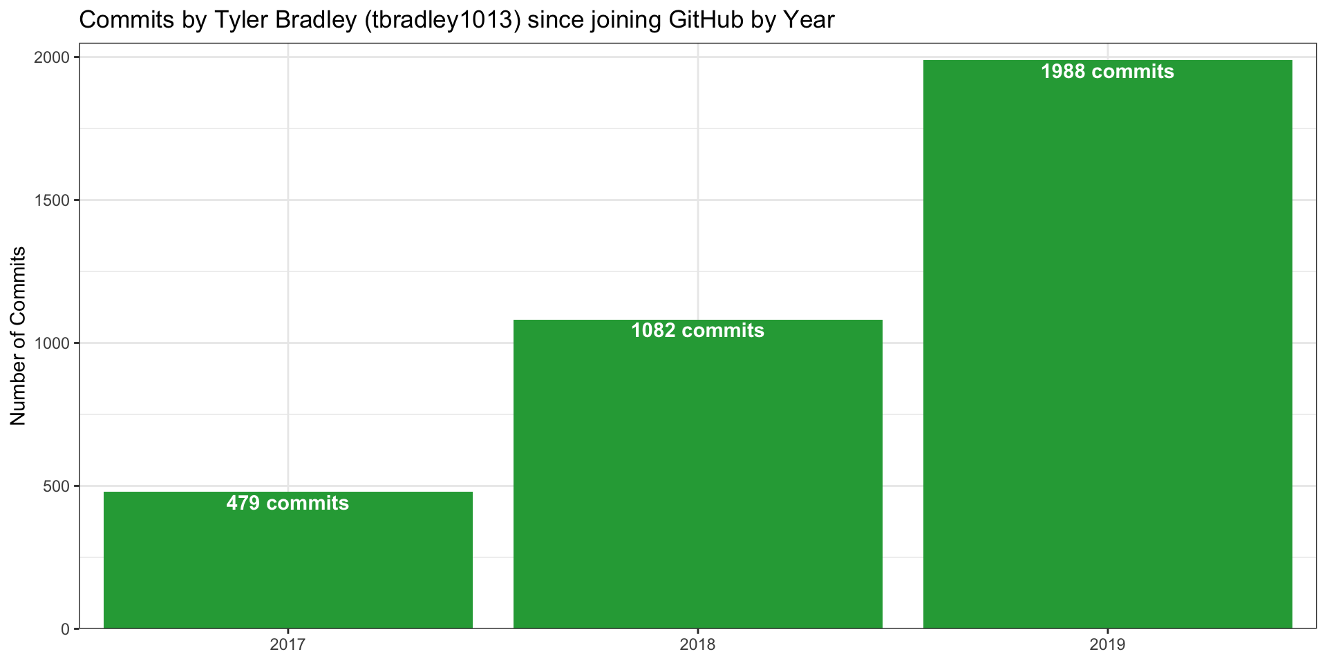
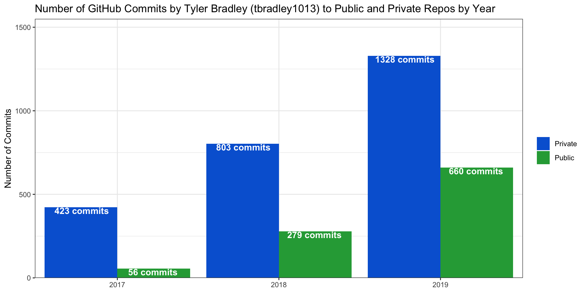
We can see that I have used GitHub more and more over the last three years, with my highest number of commits coming in 2019 (n = 1988). The same trend is true when looking at my commits to public and private repos.
my_commits  %>%
  count(year, private) %>%
  mutate(private = ifelse(private, "Private", "Public"),
         year = factor(year, levels = unique(year)),
         text_x = ifelse(private == "Private", as.numeric(year) - 0.22, as.numeric(year) + 0.22)) %>%
  ggplot(aes(year, n, fill = private)) +
  geom_col(position = "dodge") +
  geom_text(aes(text_x, n-20, label = paste(n, "commits")), color = "white", fontface = "bold") +
  theme_bw() +
  # ggsci::scale_f
  scale_fill_manual(values = c(unname(gh_pal["blue"]), unname(gh_pal["green"]))) +
  scale_y_continuous(expand = c(0, 0), limits = c(0, 1550)) +
  scale_x_discrete(expand = c(0.17, 0.17)) +
  labs(
    title = "Number of GitHub Commits by Tyler Bradley (tbradley1013) to Public and Private Repos by Year",
    y = "Number of Commits"
  ) +
  theme(
    axis.title.x = element_blank(),
    legend.title = element_blank()
  )
We can also use ggplot2 to recreate the GitHub contribution heatmap. There is a minor bit of hacking to get the axes in the desired format showing the start to the month, but it can be done like this.
my_commits %>%
  count(date, wday, year, week) %>%
  mutate(
    week = factor(week),
    wday = fct_rev(wday)
  ) %>%
  group_by(year, week) %>%
  mutate(
    min_date = floor_date(date, "week"),
    min_date = if_else(
      year(min_date) < year,
      as.Date(str_replace(min_date, as.character(year-1), "1998")),
      as.Date(str_replace(min_date, as.character(year), "1999"))
    )

  ) %>%
  ungroup() %>%
  ggplot(aes(min_date, wday, fill = n)) +
  facet_wrap(~year, ncol = 1) +
  geom_tile(width = 5, height = 0.9, color = "black") +
  theme_bw() +
  scale_y_discrete(expand = c(0,0)) +
  scale_x_date(date_breaks = "1 month", date_labels = "%b", expand = c(0, 0)) +
  labs(
    title = "Tyler Bradley's (tbradley1013) GitHub contributions heat map by year"
  ) +
  theme(
    panel.grid.major = element_blank(),
    panel.grid.minor = element_blank(),
    axis.title = element_blank(),
    legend.title = element_blank()
  ) +
  scale_fill_gradient(low = gh_pal["light_green"], high = gh_pal["green"])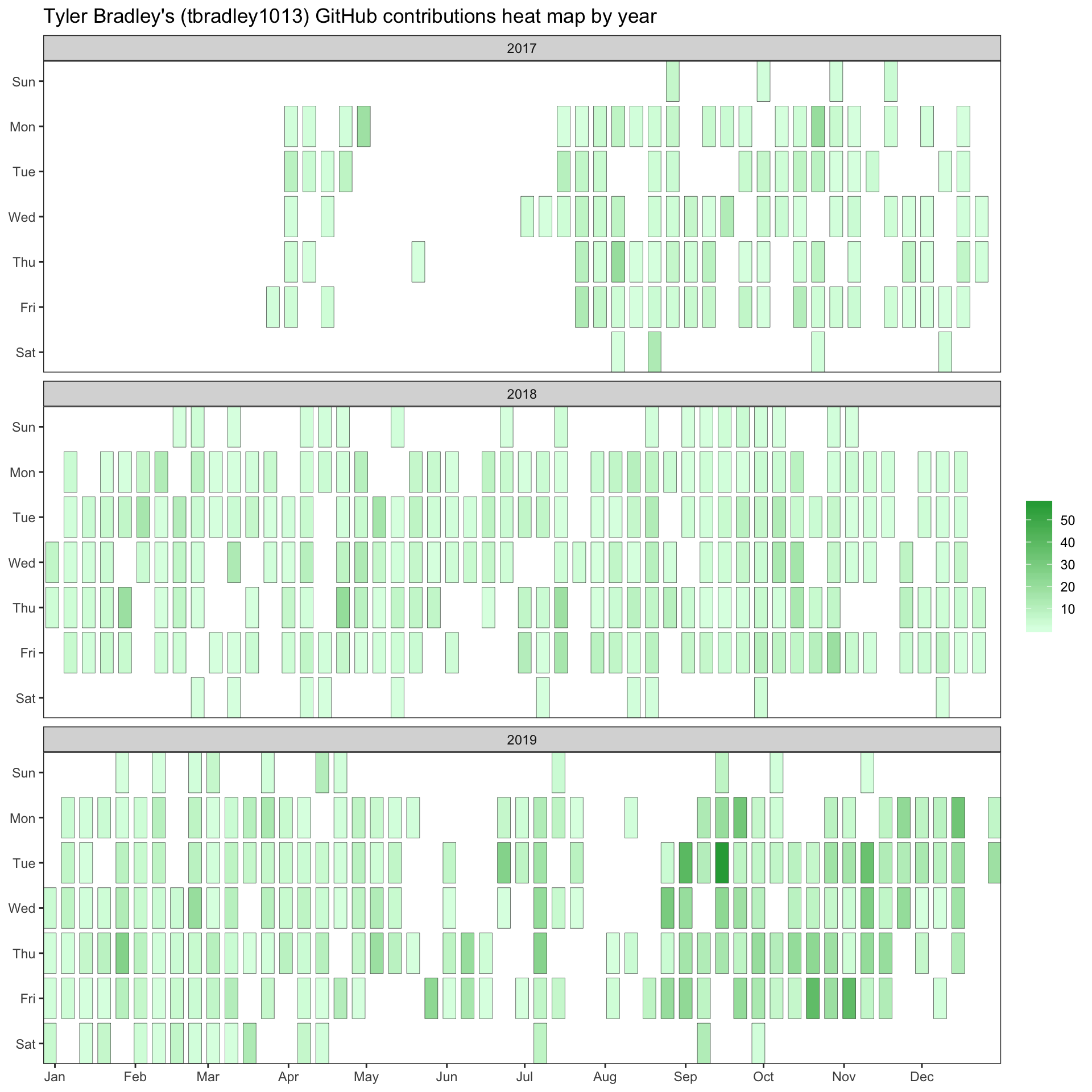
Now we can look just at the last year and see when I am the most productive according to commits. We can group the commits by the day of the week and the time of day to see if any patterns can be seen.
my_commits %>%
  filter(year == 2019) %>%
  mutate(
    hour = hour(commit_time)
  ) %>%
  count(hour) %>%
  mutate(
    text_y = ifelse(n < 50, n+5, n-5),
    text_color = ifelse(n < 50, "black", "white")
  ) %>%
  ggplot(aes(hour, n)) +
  geom_col(fill = gh_pal["green"]) +
  geom_text(aes(y = text_y, color = text_color, label = paste("n =", n)), show.legend = FALSE, size = 3) +
  theme_bw() +
  scale_x_continuous(breaks = seq(0, 23, 2), labels = seq(0, 23, 2)) +
  scale_y_continuous(expand = c(0, 0), limits = c(0, 310)) +
  scale_color_manual(values = c("black", "white")) +
  labs(
    title = "Commits by Tyler Bradley (tbradley1013) in 2019 by time of day",
    y = "Number of Commits",
    x = "Time of Day (Hour)"
  )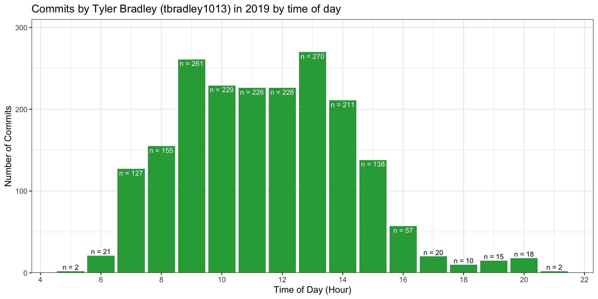
My most productive time periods are clearly between 9 am and 2 pm. Over the course of that time it appears that I am fairly consistent in my productivity. This period of productivity corresponds to the time when I am in the office at work. The time periods right outside of that window (7am-8am and 3pm-4pm) are typically the beginning and end of my work day so I am either getting my day started or wrapping things up at that point. It is clear from this figure that I don’t tend to do any work from 10pm-5am which conforms as expected with my sleep schedule.
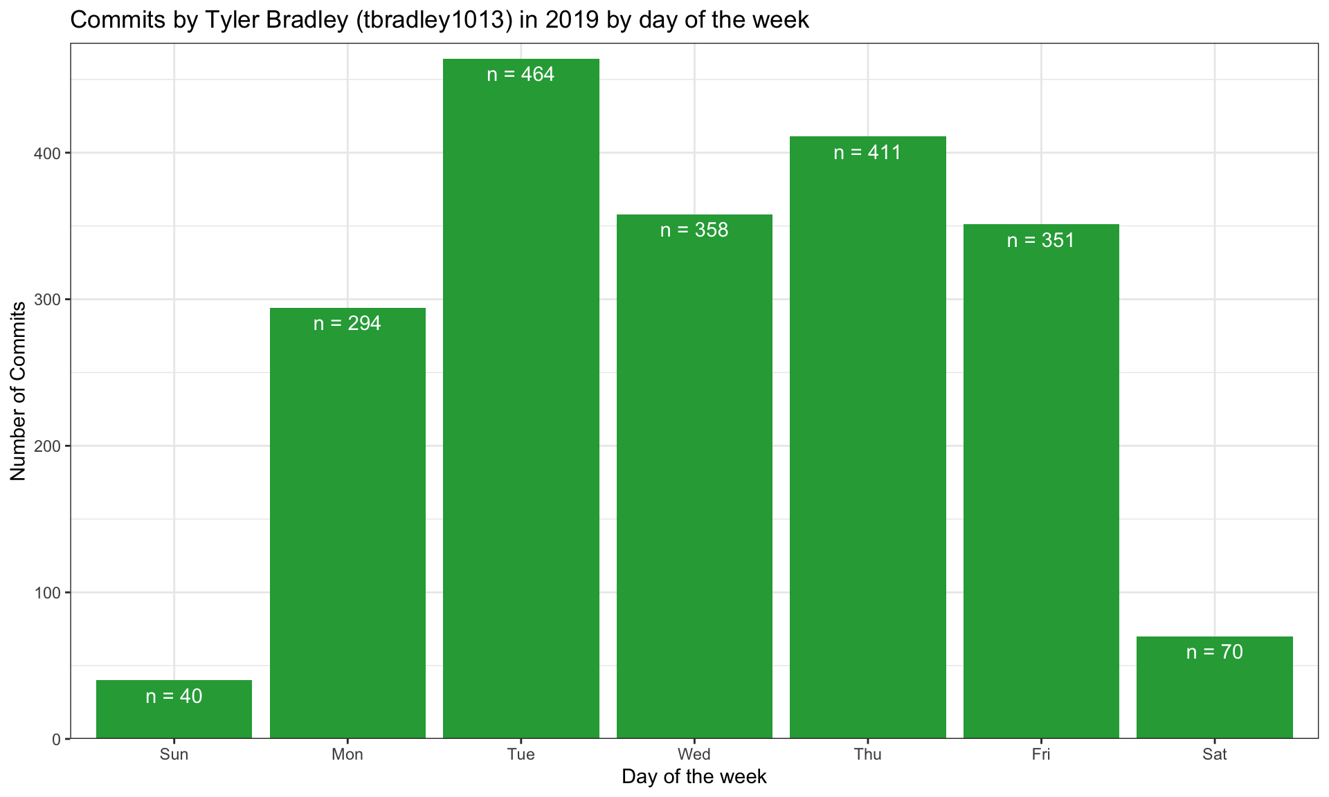
Similarly, my commits by day of the week conforms with an expected pattern that my most productive periods are when I am at work in the office Monday-Friday.
my_commits %>%
  filter(year == 2019) %>%
  count(wday) %>%
  ggplot(aes(wday, n)) +
  geom_col(fill = gh_pal["green"]) +
  geom_text(aes(y = n-10, label = paste("n =", n)), color = "white", show.legend = FALSE) +
  theme_bw() +
  scale_y_continuous(expand = c(0, 0), limits = c(0, 475)) +
  scale_color_manual(values = c("black", "white")) +
  labs(
    title = "Commits by Tyler Bradley (tbradley1013) in 2019 by day of the week",
    y = "Number of Commits",
    x = "Day of the week"
  )
Conclusion
Overall, 2019 was a very productive year for me in terms of GitHub commits! At this point, I am very committed to the git/GitHub workflow and expect that my commits will continue to either follow an upward trend or reach a plateau as I continue to take on new and exciting projects at work and in school!
The gh package allows R users to easily interact with the GitHub API and analyze how they are utilizing the tools available through GitHub.